Setup
library(ggplot2)
library(gridExtra)
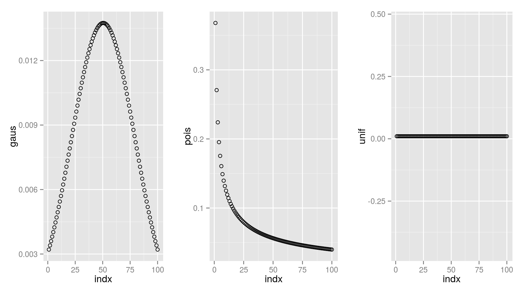
Distribution
size <- 100
vect <- seq(1, size, by=1)
m    <- mean(vect)
std  <- sqrt(var(vect))
distF <- data.frame(
  indx = vect,
  gaus = dnorm(vect, mean=m, sd=std),
  pois = dpois(vect, vect),
  unif = dunif(vect, min=1, max=size)
  )
g1 <- ggplot(data=distF, aes(x=indx, y=gaus)) +
  geom_point(shape=1) +
  guides(legend.title=element_blank())

g2 <- ggplot(data=distF, aes(x=indx, y=pois)) +
  geom_point(shape=1)

g3 <- ggplot(data=distF, aes(x=indx, y=unif)) +
  geom_point(shape=1)

grid.arrange(g1, g2, g3, ncol=3)`
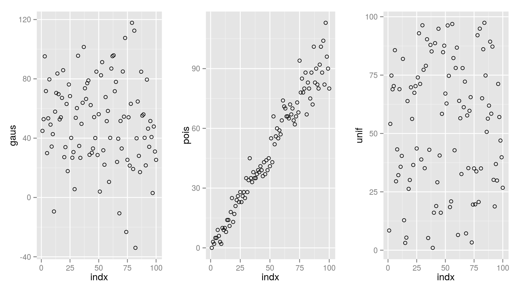
Random sampling
randF <- data.frame(
  indx = vect,
  gaus = rnorm(vect, mean=m, sd=std),
  pois = rpois(vect, vect),
  unif = runif(vect, min=1, max=size)
  )
g1 <- ggplot(data=randF, aes(x=indx, y=gaus)) +
  geom_point(shape=1)

g2 <- ggplot(data=randF, aes(x=indx, y=pois)) +
  geom_point(shape=1)

g3 <- ggplot(data=randF, aes(x=indx, y=unif)) +
  geom_point(shape=1)

grid.arrange(g1, g2, g3, ncol=3)
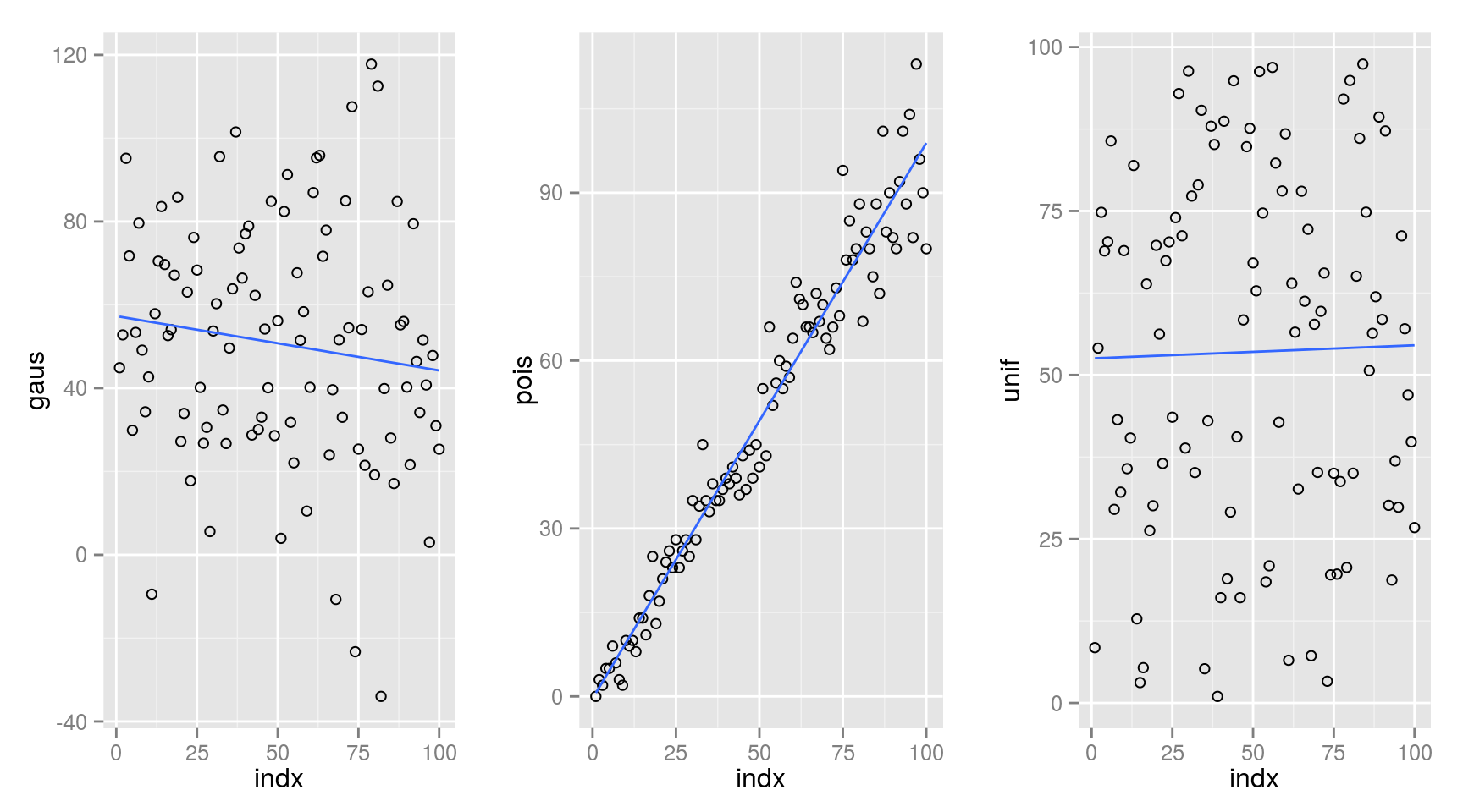
Random sampling with linear model
g1 <- ggplot(data=randF, aes(x=indx, y=gaus)) +
  geom_point(shape=1) +
  geom_smooth(method=lm, se=FALSE, fullrange=TRUE)

g2 <- ggplot(data=randF, aes(x=indx, y=pois)) +
  geom_point(shape=1) +
  geom_smooth(method=lm, se=FALSE, fullrange=TRUE)

g3 <- ggplot(data=randF, aes(x=indx, y=unif)) +
  geom_point(shape=1) +
  geom_smooth(method=lm, se=FALSE, fullrange=TRUE)

grid.arrange(g1, g2, g3, ncol=3)
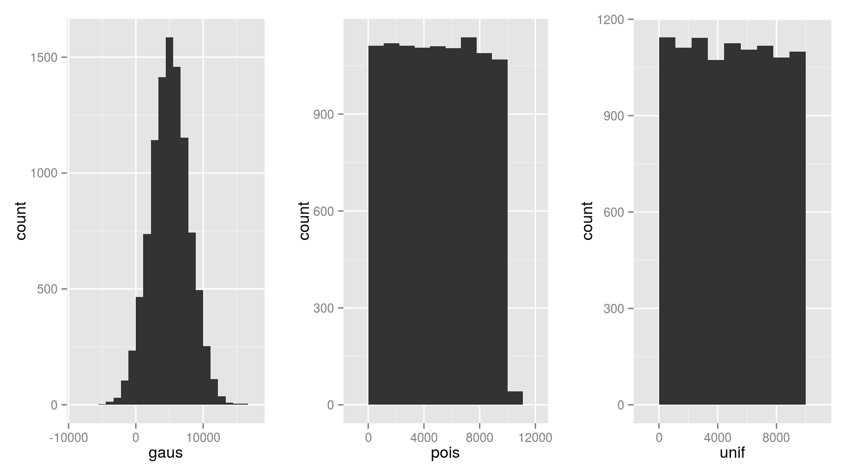
Random sampling histogram
size <- 10000
vect <- seq(1, size, by=1)
m    <- mean(vect)
std  <- sqrt(var(vect))
randF <- data.frame(
  indx = vect,
  gaus = rnorm(vect, mean=m, sd=std),
  pois = rpois(vect, vect),
  unif = runif(vect, min=1, max=size)
  )
binw <- size/9

g1 <- ggplot(data=randF, aes(x=gaus)) +
  geom_histogram(binwidth=binw)

g2 <- ggplot(data=randF, aes(x=pois)) +
  geom_histogram(binwidth=binw)

g3 <- ggplot(data=randF, aes(x=unif)) +
  geom_histogram(binwidth=binw)

grid.arrange(g1, g2, g3, ncol=3)
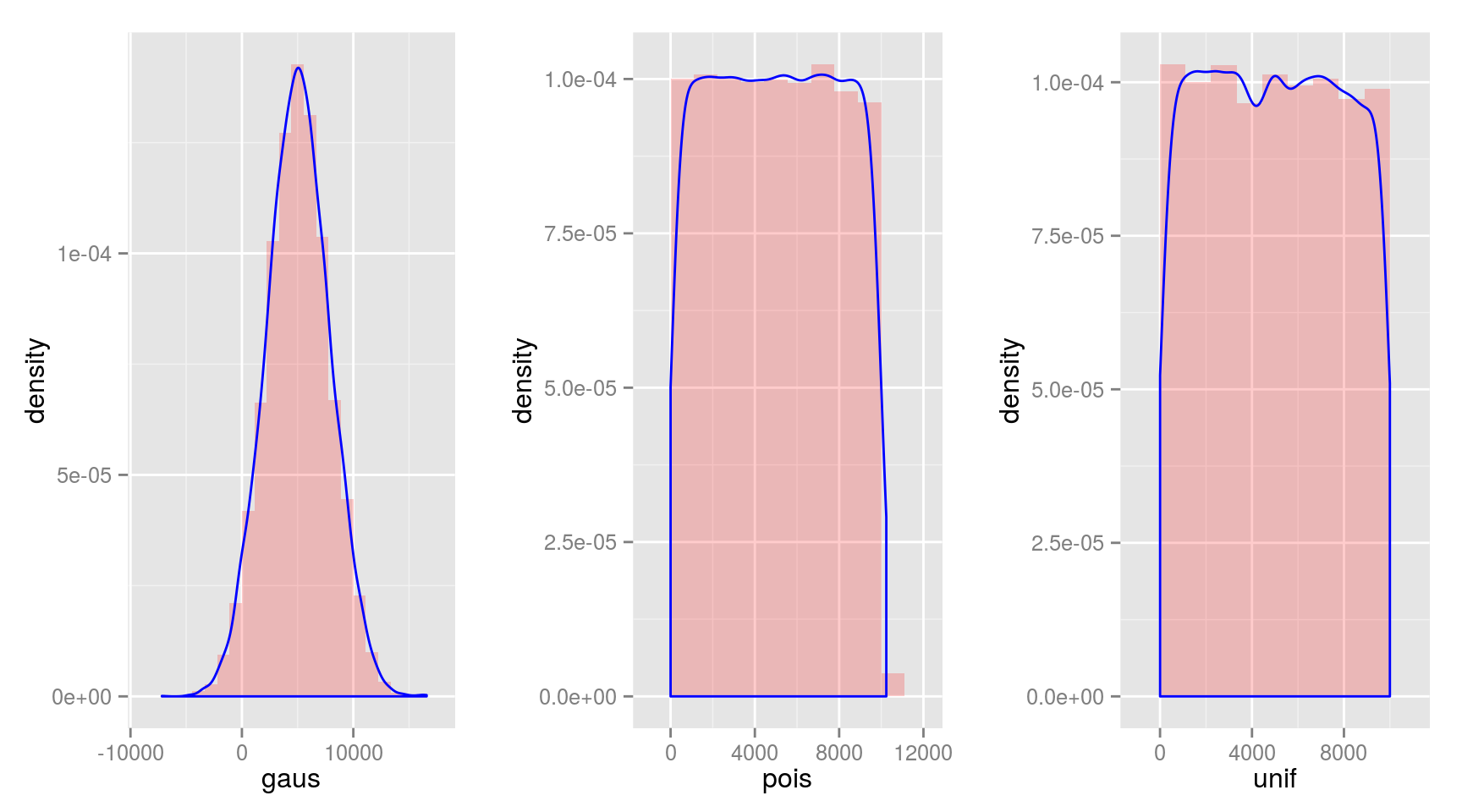
Random sampling with density
binw <- size/9

g1 <- ggplot(data=randF, aes(x=gaus)) +
  geom_histogram(aes(y = ..density..), binwidth=binw, alpha=.2, fill="red") +
  geom_density(alpha=.7, col="blue")

g2 <- ggplot(data=randF, aes(x=pois)) +
  geom_histogram(aes(y = ..density..), binwidth=binw, alpha=.2, fill="red") +
  geom_density(alpha=.7, col="blue")

g3 <- ggplot(data=randF, aes(x=unif)) +
  geom_histogram(aes(y = ..density..), binwidth=binw, alpha=.2, fill="red") +
  geom_density(alpha=.7, col="blue")

grid.arrange(g1, g2, g3, ncol=3)
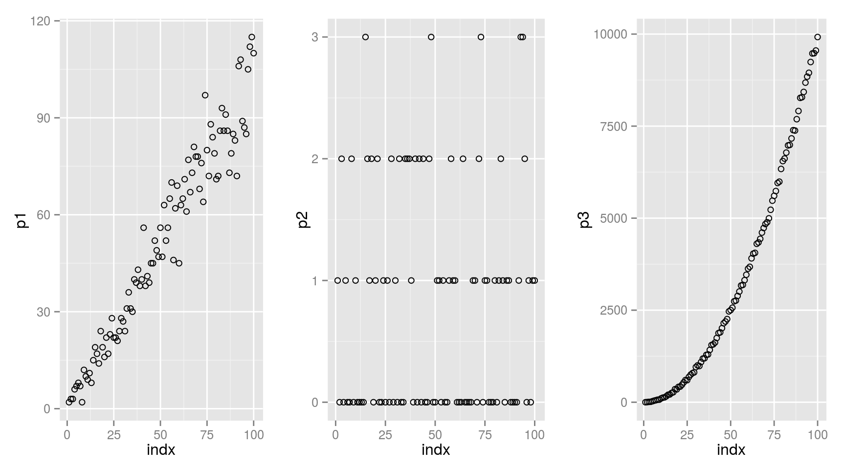
Poisson variations
size <- 100
vect <- seq(1, size, by=1)

poisF <- data.frame(
  indx = vect,
  p1   = rpois(vect, vect),
  p2   = rpois(vect, rep(1, times=size)),
  p3   = rpois(vect, vect^2)
)
g1 <- ggplot(data=poisF, aes(x=indx, y=p1)) +
  geom_point(shape=1)

g2 <- ggplot(data=poisF, aes(x=indx, y=p2)) +
  geom_point(shape=1)

g3 <- ggplot(data=poisF, aes(x=indx, y=p3)) +
  geom_point(shape=1)

grid.arrange(g1, g2, g3, ncol=3)